Docs
CM
ACP
Procédez à l'étude des données associées aux fichiers suivants : exoReg1.txt.
> reg1=read.table("exoReg1.txt")
> acp = princomp(reg1,cor=TRUE)
> acp
Call:
princomp(x = reg1, cor = TRUE)
Standard deviations:
Comp.1 Comp.2 Comp.3 Comp.4 Comp.5
1.79207900 1.25543181 0.44595569 0.10893290 0.04001203
5 variables and 13 observations.
> summary(acp)
Importance of components:
Comp.1 Comp.2 Comp.3 Comp.4 Comp.5
Standard deviation 1.7920790 1.2554318 0.44595569 0.108932897 0.0400120302
Proportion of Variance 0.6423094 0.3152218 0.03977530 0.002373275 0.0003201925
Cumulative Proportion 0.6423094 0.9575312 0.99730653 0.999679807 1.0000000000
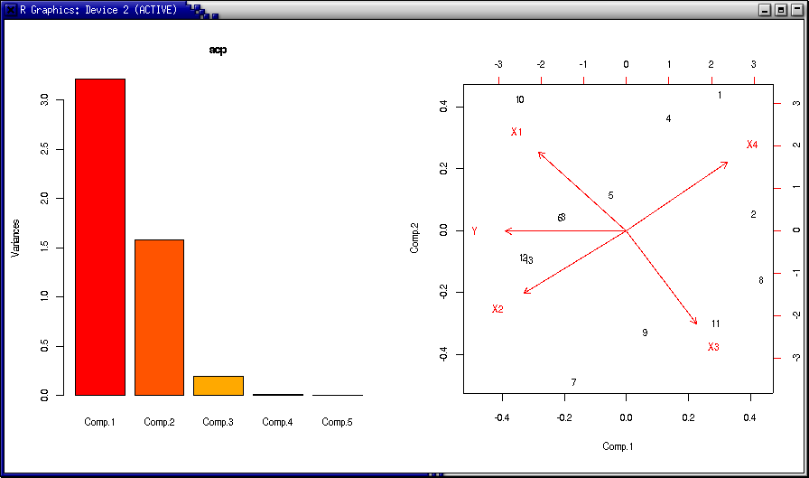
> par(mfrow=c(1,2))
> plot (acp)
> biplot(acp)
> acp$sdev
    Comp.1     Comp.2     Comp.3     Comp.4     Comp.5
1.79207900 1.25543181 0.44595569 0.10893290 0.04001203

> acp$sdev*acp$sdev
     Comp.1      Comp.2      Comp.3      Comp.4      Comp.5
3.211547154 1.576109031 0.198876476 0.011866376 0.001600963

> eigen(cor(reg1))
$values
[1] 3.211547154 1.576109031 0.198876476 0.011866376 0.001600963

$vectors
           [,1]         [,2]       [,3]        [,4]       [,5]
[1,]  0.5533800 -0.003342949  0.2106032  0.80495783 -0.0380602
[2,]  0.4011658  0.512413468  0.5812090 -0.41341229  0.2603552
[3,]  0.4682512 -0.409678782 -0.3896683 -0.19084641  0.6516444
[4,] -0.3189779 -0.607968833  0.6746443  0.05282357  0.2658790
[5,] -0.4602504  0.447167145 -0.1041923  0.37672337  0.6598747

> acp$loadings

Loadings:
   Comp.1 Comp.2 Comp.3 Comp.4 Comp.5
Y  -0.553         0.211  0.805
X1 -0.401  0.512  0.581 -0.413  0.260
X2 -0.468 -0.410 -0.390 -0.191  0.652
X3  0.319 -0.608  0.675         0.266
X4  0.460  0.447 -0.104  0.377  0.660

               Comp.1 Comp.2 Comp.3 Comp.4 Comp.5
SS loadings       1.0    1.0    1.0    1.0    1.0
Proportion Var    0.2    0.2    0.2    0.2    0.2
Cumulative Var    0.2    0.4    0.6    0.8    1.0

> acp$center
        Y        X1        X2        X3        X4
95.438462  7.461538 48.153846 11.769231 30.000000

> acp$scale
        Y        X1        X2        X3        X4
14.431138  5.651622 14.950411  6.153846 16.081523

> acp$n.obs
[1] 13

> acp$scores

         Comp.1     Comp.2      Comp.3       Comp.4      Comp.5
  1   1.9357055  1.9733074 -0.54408887  0.025000659  0.03952149
  2   2.6585707  0.2364222 -0.25919227  0.092331415 -0.03498866
  3  -1.3182914  0.1980815 -0.05971679 -0.131317652 -0.09155472
  4   0.8778336  1.6377820  0.17323706 -0.111200481 -0.02929345
  5  -0.3185821  0.5060423 -0.79289121  0.031163656  0.01900113
  6  -1.3657941  0.1811666  0.13452792  0.210201419 -0.02279333
  7  -1.0930548 -2.2163607 -0.21936861 -0.077556747  0.01231682
  8   2.8065014 -0.7319342  0.47873229 -0.172077644  0.03163279
  9   0.3882477 -1.4928554 -0.01325269  0.060519403 -0.04967684
  10 -2.2266661  1.9107006  0.89514664  0.005335703  0.01961902
  11  1.8569418 -1.3580321  0.58348404  0.117665351  0.02698841
  12 -2.1537352 -0.3992735 -0.02755253  0.064219514  0.03552010
  13 -2.0476770 -0.4450468 -0.34906497 -0.114284596  0.04370725
- acp$sdev :
- les écarts-types correspondent à la racine carré des valeurs propres
- proportion of variance :
- exprimée par les valeurs propres (eigen values en anglais)
- acp$loading :
- Matrice de rotation simplifiée, obtenue avec les vecteurs propres
- acp$center :
- centres associés à la matrice de rotation utilisée pour changer de repère
- acp$scale :
- echelle
- acp$scores
- Coordonnées des exemples dans le nouveau repère
Exercice
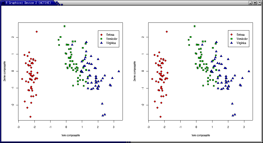
Réaliser une ACP sur les données iris et comparer les projections obtenues avec les deux méthodes sur les données iris :
> data(iris)
> irisACP = princomp(iris[1:4],cor=TRUE)
> irisACP2 = prcomp(iris[1:4],scale=TRUE)

> par(mfrow=c(1,2))

> plot(irisACP$scores[,1],irisACP$scores[,2],pch=c(rep(21,times=50),rep(22,times=50),rep(24,times=50)),
bg=c("red", "green3", "blue")[unclass(iris$Species)],xlab="1ere composante",ylab="2eme composante")
> legend(2.,2.4,c("Setosa","Versicolor","Virginica"),pch=c(21,22,24),pt.bg=c("red","green","blue"))

> plot(irisACP2$x[,1],irisACP2$x[,2],pch=c(rep(21,times=50),rep(22,times=50),rep(24,times=50)),
bg=c("red", "green3", "blue")[unclass(iris$Species)],xlab="1ere composante",ylab="2eme composante")
> legend(2.,2.4,c("Setosa","Versicolor","Virginica"),pch=c(21,22,24),pt.bg=c("red","green","blue"))